- Context
- I. The Problems with Observational Studies
- II. A Solution: Matching
- III. Sensitivity Analysis
- IV. Conclusion
- Resources
Due to the lack of random assignment to treatment groups in observational studies, omitted variable bias can affect treatment effect estimates. One can therefore question results of regression analyses for such studies, and sensitivity analysis allows to quantify the impact of potential omitted variables. In the paper ‘Housing, Health and Happiness’, the matching between treatment and control is not fully transparent, and the lack of sensitivity analysis does not allow to measure its performance.
In this extension, we propose to conduct a robustness check to verify the matching through a sensitivity analysis for various matching methods, in order to assess the bias needed to change the results significantly. Specifically, a similar matching as proposed in the paper and a propensity score matching are studied. Finally, analysis of the regressions performed in the paper for the different matchings can be carried out.
Context
In the paper ‘Housing, Health and Happiness’, the aim is to measure the impact of replacing dirt floors with cement floors in Mexico, on health and welfare of young children and their mothers. A large-scale program called Piso Firme offered households up to 50m² of cement floor. It was established by the Mexican government in $2000$ in the State of Coahuila first, then in $2004$ in the state of Durango. The study observes the evolution of two populations in two twin cities: Gomez Palacios and Lerdo, State of Coahuila (group control) and Torreon, State of Durango (group treatment). They are geographically close but the beginning of the program implementation differ as they are in two different states. They proceded in three steps: verification that control and treatment groups are well balanced, estimation of the program impact using a linear regression model and examination of the robustness of the results. Their verification showed that both control and treatment groups were balanced on all levels before the program. Their conclusion was that the Piso Firme program improved health and welfare of young children and their parents. The cement floors significantly reduced the number of cases of parasitic infestations, diarrhea, anemia and then improved the health and cognitive development of the children. They also increased happiness and quality of life of adults as well as decreased depression.
I. The Problems with Observational Studies
Randomised ?
In an ideal randomised trial, the treatment assignment would be randomly decided, i.e. equivalent to a $50/50$ coin flip. Therefore, if we assume the trial is actually randomised, the distribution of our covariates will be the same in both groups, i.e. the covariates are said to be balanced. In this case, the control and treatment groups are indistinguishable. Thus, if the outcome between different treatment groups end up differing, it will not be because of differences in the covariates defining the groups, it will be because of the treatment.
However, as it is not always possible to perform a randomised trial (either unethical, impractical, too expensive, …), observational studies are conducted, where there is no intervention in the treatment assignment and retrospective data is observed. This is the case of the ‘Housing, Health and Happiness’ paper. Indeed, data is collected from census and surveys a posteriori and the researchers cannot control the conditions under which samples are distributed. This might lead to a potential problem as the decision of which subjects receive the treatment is not entirely random and thus a potential source of bias.
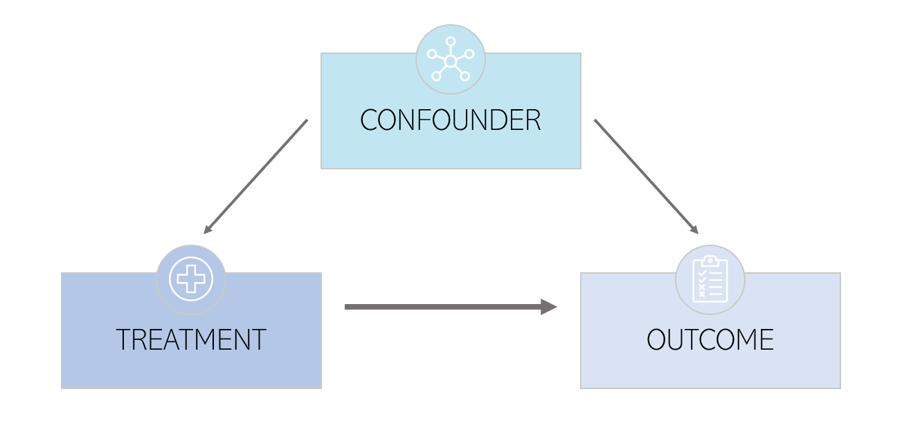
To be more precise, subjects are selected to be treated and the treatment assignment and the outcome may be caused by the same hidden covariate. For observational studies, the distribution of variables will typically differ between treatment and control group, as it is not a randomised trial. The goal of the study is to determine the extent to which the variables defining households before the start of the programme impact the outcome instead of the Piso Firme program. However, sometimes the measured covariates are not directly responsible for the differences in outcome. There may indeed be other covariates that were not measured but are in fact important in the chain of cause and effect. These variables that affect both treatment attribution and outcome are called confounders, as seen on the diagram below. In observational studies, an important assumption in the estimation of causal effect is the ignorability assumption : given pre-treatment covariates, treatment assignment is independent of the potential outcome, also known as the “no unmeasured confounders’ assumption”.
Balanced ?
We can start by analysing the distribution and properties of the variables from the $2000$ Census, which are the pre-treatment variables. In the dataset, they correspond to the variables beginning in ‘C_’. Following the results given in Table 2 of the paper, we can compute the mean values of treatment and control, as well as the mean difference by aggregating at census block level. In the paper, this is what they use as evidence to show that the data is balanced with their matching. The authors do not apply any statistical test to demonstrate their results, so we decide to apply a statistical test to check wether the variables are balanced or not. To assess whether balance is achieved between treatment and control, a useful tool is the standardised mean differences (SMD), which is calculated by the difference in the means between the two groups divided by the pooled standard deviation :
where $ \bar{X_t} $, $ \bar{X_c} $ denote the mean of that feature for the treatment and control group respectively. We will use the absolute value of this number. The variables $s_{t}$, $s_{c}$ denote the standard deviation of that feature for the treatment and control group respectively.
We can calculate the standardised mean differences for every feature, and if our calculated SMD is $1$, then that means there’s a $1$ standard deviation difference in means. After computing this measurement for all of our features, there is a rule of thumb that is commonly used to determine whether that feature is balanced or not (similar to the $0.05$ for $p$-value idea, which we can also use with a $t$-test) :
- $\mathrm{SMD} < 0.1$ : The covariate is balanced. We can assume a randomised trial.
- $0.1 < \mathrm{SMD} < 0.2$ : The covariate is not necessarily balanced, but the discrepancy is small enough to be ignored.
- $\mathrm{SMD} > 0.2$ : The covariate is considered seriously imbalanced.
The graph below shows the $\mathrm{SMD}$ value for different variables, computed using the paper’s original dataset. We can see that about $36 \%$ of the variables are such that $\mathrm{SMD} < 0.1$ and $63 \%$ of the variables are such that $\mathrm{SMD} < 0.2$. It is clear that the distributions of the pre-treatment variables between treatment and control sets are not balanced for most of the variables.
II. A Solution: Matching
Theory and background
To solve the issue of the difference in variables distribution between control and treatment group, matching is performed. The idea is to match individuals in the treated group with similar individuals in the control group for the covariates. In the ideal case, we would like to find for each sample in the treatment group, an identical sample in the control group in terms of pre-treatment covariates. This is generally impossible, but fortunately, finding similar sample in the control group is enough. The condition is that the two samples in the matched pair have a probability of receiving the treatment that is as close as possible. This is not an exact matching as the paired samples can be slightly diffferent, but the overall distribution of each pre-treatment variable is balanced between the groups - this is known as stochastic balance. Matching is a technique that attempts to control for confounding and make an observational study more like a randomised trial. It enables a comparison of outcomes among treated and control samples to estimate the effect of the treatment and reducing the bias due to a potential confounder, and it can be done in different ways.
Replicating the paper’s matching method
In the paper they use the $\bold{L_{\infty}}$ norm. The pairs are created based on $4$ pre-treatment variables :
- C_blocksdirtfloor : Proportion of blocks with houses that has dirt floors
- C_HHdirtfloor : Proportion of households with dirt floors
- C_child05 : Average number of children between $0$ and $5$ years
- C_households : Number of households
They are therefore matching on observed covariates. The idea is to minimise the $L_{\infty}$ distance to match the pairs of control and treatment data points. The $L_{\infty}$ distance is defined as the maximum of the absolute value of the differences between the variables for each pair of treatment and control blocks. We can compute the $L_{\infty}$ distance between each possible pair of treated and control data points and minimise to obtain the final matching.
In practice, we construct a bipartite graph. Each node represents a sample; treated samples are on one side of the graph and control samples are on the other side. The edges link one control and one treated sample, weighted with the $L_{\infty}$ norm. The aim is to minimise the norm over the matching. Thus the algorithm finds the best set of matched pairs such that the norm is minimised.
The figure below represents the distributions of one of the 4 variables used for matching (C_blocksdirtfloor), comparing before and after the matching step. We can therefore compare the distribution of the treated and control subsets. The histograms partially overlap, so the distributions are quite similar both before and after matching, with a slight decrease in the distribution of controls after matching. Indeed, as more control data points are available than treatment, the matching step will usually match all treatments with a subset of controls, and this is observed here as all treatment data points are matched (no difference in the distributions of treatment before and after matching).
The next figure is the graphical result of a $\mathrm{SMD}$ applied on the census variables after the matching step. We can see that the value of the $\mathrm{SMD}$ has slightly decreased for the 4 variables used in the matching. However, C_blocksdirtfloor and C_child05 are still unbalanced as their $\mathrm{SMD}$ value is above $0.2$. In general, the variables with a very high $\mathrm{SMD}$ before the matching still have a high $\mathrm{SMD}$ after the matching, and the value has actually increased for some of them. Therefore, by looking at the $\mathrm{SMD}$ test, it seems that the matching is not efficient. This could be due to the fact that only 4 of the pre-treatment variables are used to match the data points, and we indeed observe an average of 7% decrease in the SMD values for the 4 matching variables. Moreover, this could be explained by the fact that the data used for matching was the data set provided by the authors to recreate the results of their findings, and therefore already corresponds to matched samples. Indeed, the number of control group varibales is relatively low and similar to the treatment group in the first place, so the matching did not significantly change the number of data points. Therefore, significant changes in the distributions and SMD are not expected.
Propensity score matching
Another method used for matching is based on what is called propensity score. In this case, the goal is that the two samples of the pair have the same probability to be treated. For subject $l$, the probability of being treated given full knowledge of the world is :
with $Z_l$ the treatment assignment, $r_{Cl}$ the response if the subject is control, $r_{Tl}$ the response if the subject is treated, $\bold{x_{l}}$ the observed covariates and $u_{l}$ the unobserved covariates. Instead of matching on observed covariates directly, the idea is to reduce the information of all the pre-treatment covariates to one single number called the propensity score. Of course, the formula above is idealistic as we don’t know all these variables. In practice, we can estimate $\pi_{l}$ for every sample using a logistic regression on $\bold{x_{l}}$. By doing so, the samples with equal propensity score are guaranted to have equal distributions of observed variables. The samples in the same pair might not have equal $\bold{x}$, but total treatment and control groups will have the same distribution.
In practice, we construct a bipartite graph as explained above for the matching with $L_{\infty}$ norm. The edges are now weighted with the difference of similarity score. The similarity is defined as 1 minus the difference of propensity score, and we want to minimise the difference of propensity scores between the pairs. Equivalently, we can maximise the similarity between the pairs. The algorithm therefore finds the matching that maximises the overall similarity.
Two different propensity score matchings are applied in this study. The first one takes into accout only the $4$ variables used in the paper’s matching, and the second one is a propensity score matching using all the pre-treatment census variables. The figures below illustrate the distribution of the propensity scores before and after the matching, when using all census variables. There is little overlap in the distribution of propensity scores matching for the treatment and control groups, and the distributions do not change significantly before and after matching. The intuition we could propose is that if the additional variables included in the propensity score are highly correlated with which sample is treated and which one is not, it means that they can potentially cause a lot of confounding. Therefore, we would not want to exclude them since this study aims precisely at assessing their impact. Nevertheless, as the matching does not seem to be effective, we can improve it by matching only observations with similar propensities through the addition of a threshold on the accepted value difference. For example, by adding a similarity threshold of 0.99, the obtained distributions have greater overlap after matching, as expected.
The figure above shows the propensity score distribution before matching. Below, the two matching methods are applied and the results on the distributions for treatment and control groups can be observed. When no threshold is applied, the control group distribution decreased slightly, as was observed with the $L_{\infty}$ norm matching. When the 0.99 similarity threshold is applied, the distributions match very closely, as expected.
The results of the $\mathrm{SMD}$ test are shown below for both propensity score matching methods, and they are similar to the ones of the paper’s matching. In fact, the matching does not seem to be more effective than using the $L_{\infty}$ norm, and for some variables the SMD increases significantly. One could therefore conclude that in terms of balancing the pre-treatment covariates of the study, propensity score does not seem to be an effective solution.
III. Sensitivity Analysis
Theory and background
Matching can improve the veracity of the results. It ensures that similar samples are compared, i.e. they are similar in terms of observed variables. Nevertheless, there might be some unobserved covariates that highly differ between the two samples. In other words, a naive model assumes that the probability to be treated was $0.5$ inside the pairs treated-control. However, there might exists an unmeasured confounder that could unbalance this probability by favouring one sample or the other. Sensitivity analysis allows to quantify the degree to which the naive model is wrong.
“In treatment-control pairs matched, the chance that the first person in pair $p$ is treated is $\theta_{p} = 0.5$ under the assumption that treatment assignment is ignorable. What if that assumption is wrong ?” Paul R. Rosenbaum, Observation and experiment
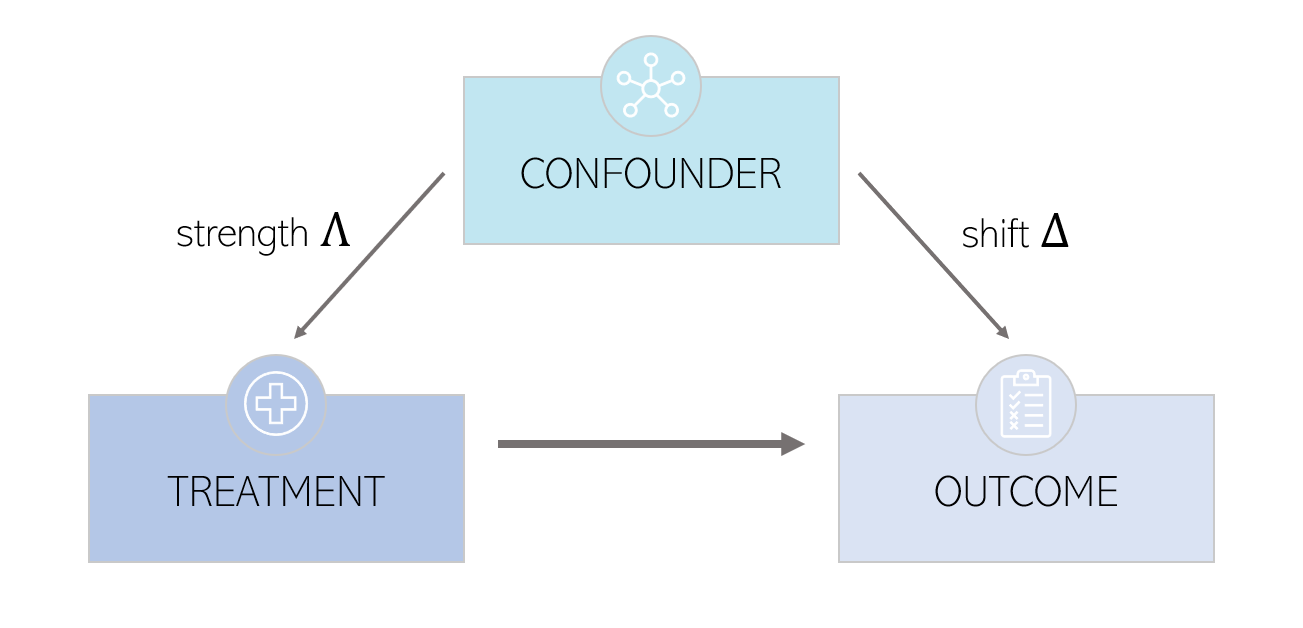
The intuition is that the naive model would be wrong if there exists a confounder sufficiently important to modify the probability of being treated by a certain amount. Let’s be more precise - the model assumes that the odds of two similar data points (i.e. very similar observed covariates) are bounded by a factor $\Gamma$ : $ \frac{1}{\Gamma} \leq \frac{\pi_k(1 - \pi_k)}{\pi_l(1 - \pi_l)} \leq \Gamma $. For example, if $\Gamma = 3$, the odds ratio is comprised between $1/3$ and $3$, and the probabilty of being treated is comprised between $0.25$ and $0.75$.
For each value of $\Gamma$, we use a statistical test with the following hypotheses :
- $H_0$ : No treatment effect on the model.
- $H_1$ : A treatment effect on the model.
If the $p$-value $< 0.05$, we can reject the null hypothesis $H_0$ of no treatment effect. We start with $\Gamma = 1$ and then increase its value. Under the null hypothesis, increasing $\Gamma$ increases the $p$-value. Finding the smallest $\Gamma$ for which $p > 0.05$ corresponds to finding by how much would the probability have to depart from $0.5$ to obtain a $p$-value above $0.05$ so that the hypothesis of no treatment effect cannot be rejected. For example, if we obtain $p > 0.05$ for $\Gamma > 6$, then the odds of being treated would need to be $6$ times higher for two people with same covariates. Therefore, estimating a value for $\Gamma$ allows to evaluate the likelihood of a potential hidden covariate and the consequence of this covariate on the results.
In practice, we use in this work the sensitivitymv R library and more specifically senmv function. This would allow us to evaluate the robustness of the model towards the bias between the paper assignment and a randomised one.
Amplification of Sensitivity Analysis
The question is now to discuss the possibility of the existence of an unobserved covariate. Are there other unmeasured covariates that could have an impact on the outcomes of the models ? Indeed, so far we have shown that sensitivity analysis can help quantify the bias needed to invalidate the rejection of the no treatment effect hypothesis, but it does not yet tell us anything about the nature or existence of confounders.
In order to do so, we will need to go further and decompose $\Gamma$ into two parameters : $(\Lambda, \Delta)$. These parameters are defined by : $\Gamma = \frac{\Lambda \Delta + 1}{\Lambda + \Delta}$. For each value of $\Gamma$, we can draw a graph of $\Delta$ as a function of $\Lambda$.
$\Delta$ is called the
Results - Sensitivity analysis of the different matching methods
The figure below shows the results in terms of the value of $\Gamma$ for the different matchings : the paper’s matching method using $L_{\infty}$ norm, a propensity score matching using all the variables of the census and a propensity score matching using only the four variables used in the paper. The displayed value of $\Gamma$ is the smallest value for which the $p$-value of the statistical test reaches the significance level of $0.05$. We can see that the propensity score matching with all the variables performs overall slightly worse than the two other matchings. The results are uneven among the different outcomes. We can observe that the outcomes describing the presence of cement floor in the different rooms of the house (Table 4 of the original paper) are the less sensitive to bias, followed by the satisfaction outcomes (Table 6). For S_pss and S_cesds, a $p$-value $> 0.05$ is reached for $\Gamma = 1$, which means not only these outcomes are extremely sensitive to bias, but we cannot reject the null hypothesis of no treatment effect. This result is obtained for the four different matchings. S_pss and S_cesds are the outcomes measuring the percieved stress scale and the depression scale respectively. These results could be explained by the fact that the outcomes measuring the fraction of cement floors in the rooms are more easily measured as they are a physical change, compared to the stress or depression that are mental states and therefore more subjective. We can also compare the matchings with each other. The propensity score matching using only four pre-treatment variables has the best performance as $\Gamma$ is overall higher using this method. We can see that the propensity score matching using a threshold leads to more sensitive results despite the better balance in terms of distribution of propensity score. Also, the fact of including all the variables in the estimation of the propensity score doesn’t improve the performance. Indeed, some studies suggest that including irrelevant covariates in the propensity model might reduce its efficiency [1]. In particular, discarding variables that are related to treatment but not to outcomes doesn’t improve balance or reduce bias and might even make matching more difficult [2].
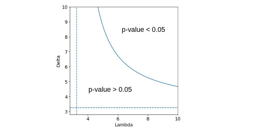
Let’s concentrate on the outcome S_shcementfloor. We measure a sensitivity of $\Gamma = 3.25$ using the matching of the paper. This corresponds to a probability of treatment comprised in $[\frac{1}{1 + \Gamma}, \frac{\Gamma}{1 + \Gamma} ] = [0.23, 0.76 ]$ which would violate the hypothesis of randomised treatment assignment. Furthermore, to put into question the conclusion of a treatment effect, we would need to find an unmeasured covariate that would influence the treatment probability such that the odds of being treated would be $3.25$ times higher for two people with same measured covariates. The next step is the amplification of the sensitivity analysis. The result is shown in the graph below. All combinaisons $(\Lambda, \Delta)$ such that $\Gamma = 3.25$ form the blue curve. The vertical and horizontal dashed lines corresponds to $\Gamma = 3.25$, which is also the asymptotes of the curve, when taking one of the parameters going to $\infty$. All combinations above the curve lead to $p < 0.05$ which means that the treatment has significant effects. On the opposite, all combinations below the curve lead to $p > 0.05$ which means that there are no significant effects of the treatment. Let’s take an example : $(\Lambda, \Delta) = (6, 7)$ corresponds to an unobserved covariate that would multiplie by $6$ the odds of treatment and multiplies the odds of a positive pair difference in the outcomes by $7$. Overall, the results show that the cement floor outcome variables are less sensitive to bias, whilst the satisfaction and mental health outcomes are sensitive to small biases.
Further analysis - Influencial Regressors in the Regression Analysis
As previously discussed, omitted variable bias can affect treatment effect estimates obtained from observational data due to the lack of random assignment to treatment groups. Sensitivity analyses adjust these estimates to quantify the impact of the non-randomised assignement and the potential omitted variables. As a further step in our sensitivity analysis, we could investigate which outcomes to consider specifically for the sensitivity analysis, and to do so we can use the available data to establish reference points for speculation about omitted confounders. For example, we can look at the effect of regressors used in the linear regression models proposed in the paper on $R^2$, a statistical measure that represents the proportion of the variance for a dependent variable that is explained by an independent variable or variables in a regression model. So, if the $R^2$ of a model is $0.50$, then approximately half of the observed variation can be explained by the model’s inputs.
To quantify this effect, we can isolate each variable used as regressors in the models and see the change incurred in $R^2$ when the regressors are not included in the model. This enables a classification of the most predictive regressors in terms of $R^2$. Indeed, the difference in $R^2$ corresponds to the bias that would have been incurred by omitting said variable in the model. We can then use this information to select the outcome variables which will be studied further in the sensitivity analysis of the matching, similarly to what was proposed above. The proportionate reduction in unexplained variance (named $\rho^2$) when $X$ is added as a regressor can be computed as follows:
This is equivalent to saying that the square of the bias due to omitting a covariate is linear in the fraction by which that covariate would reduce unexplained variance. The figures below show the results obtained for the regressors of model 3 in the paper, for Tables 4 and 6. We observe that the outcome variables S_waterhouse, S_headeduc, S_HHpeople are the most predicting in for the studied variables in Tables 4. For Table 6, S_electricity, S_waterhouse, S_garbage are the most important in terms of changes to the unexplained variance.
Using these results, we can look at the sensitivity of these outcomes in terms of $\Gamma$. It turns out that applying the same methodology as the sensitivity analysis of the regressed outcomes, we find that all 5 variables have higher $p$-values than 0.05 for $\Gamma = 1$, which shows that these for these outcomes we cannot reject the null hypothesis of no treatment effect.
IV. Conclusion
The methodology presented in this study allowed to further check the robustness of the results presented in the paper ‘Housing, Health and Happiness’. As the original paper didn’t contain any statistical test to check the balance of the treatment and control groups, SMD was used to verify the balance and various matching methods were tested to attempt to improve overall balance. Moreover, a sensitivity analyis assessing bias and the effect of confounders was carried out.
To conclude the findings of this extension study on the paper, our results show that:
-
Overall, the results of the paper for Tables 4 and 6 are indeed sensitive to bias, especially for the outcomes linked to mental health and satisfaction. The cement floor outcomes are not sensitive to small biases, satisfaction outcomes are sensitive to small biases and the hypothesis of an effect of treatment on mental health outcomes is put into question.
-
Propensity score matching does not seem to improve the balance of the data sets, which could point towards potential weaknesses of the method. Using all measured covariates to estimate the propensity score does not seem to be the best strategy, even though we could think that it would bring more knowledge to the score. Carefully selecting some of variables that are related to the outcomes might lead to improvements.
-
The SMD was not improved through the various matching methods. This could be due to the fact that the control set available is already matched, and so to further confirm the results shown above it would be ideal to have the initial control set that is bigger and not already matched. In that case, the matching would likely have been more efficient.
-
The most important variables in the data set in terms of predicting power for the studied regression models are very sensitive to bias, and we cannot reject the null hypothesis of no treatment effect for those outcomes.
To further this analysis, which has proved to be insightful in determining the robustness and validity of results presented in this observational studies, we could apply the same methodology to the outcomes describing the health of the children : S_diarrhea, S_anemia, S_S_mccdts and S_pbdypct, which were not presented here.